Playing with numpy and image processing in Python, I was wondering if it would be possible to simulate the look of old analogue video. This post describes how i have achieved something that looks sortof right. I'll provide code examples. Those who are more versed in numpy and other scientific libraries may find them inefficient, but I'm not a Python programmer, so bear with me.
Numpy keeps the images in memory in the form of a three dimensional array (for RGB images) or two dimensional (for monochrome images). This is how you load an RGB image into memory and then convert it to black and white using the Rec. 709 RGB coefficients. The color conversion topic is covered in depth in this post.
import imageio
import sys

# Rec.709 Luma calculation coefficients
COEF_R = 0.2126
COEF_G = 0.7152
COEF_B = 0.0722

if(len(sys.argv) != 2):
    print("Usage: " + sys.argv[0] + "  ")
    exit(1)

impath = sys.argv[1]
imag = imageio.imread(impath)

# Create a B/W version of the image
luma = imag[:, :, 0] * COEF_R + imag[:, :, 1] * COEF_G + imag[:, :, 2] * COEF_B
After you have loaded the image and calculated its luminance data, you can display it like this
fig, plots = plt.subplots(1, 2, squeeze=True,
                          gridspec_kw={"hspace": 0.5, "wspace":0.7},
                          constrained_layout=True,
                          figsize= (20, 20),)

plotin = plots[0].imshow(imag, cmap="Greys_r")
plots[0].set_title("Input")

plotout = plots[1].imshow(luma, cmap="Greys_r")
plots[1].set_title("Output")

plt.show()
Congratulations. You have just made your first image processing script! The full source file is bw-display.py
I decided to focus on the black and white video in this example, however adding color mangling should not be too difficult. My script simulates low bandwidth cabling and reflections of the signal at cable ends
As stated previously, the signal is encoded libe-by-line. A very sharp brightness transition, for example a person in a bright shirt standing on a dark background, or, as in the image above, an edge of a window on a computer desktop, would produce a very sharp voltage transition, a steep edge in a video signal that consists of some high frequency components. Depending on the signal bandwidth, the higher frequency components may be lost, causing the edge to become softer, thus blurring the brightness transision in the output image.
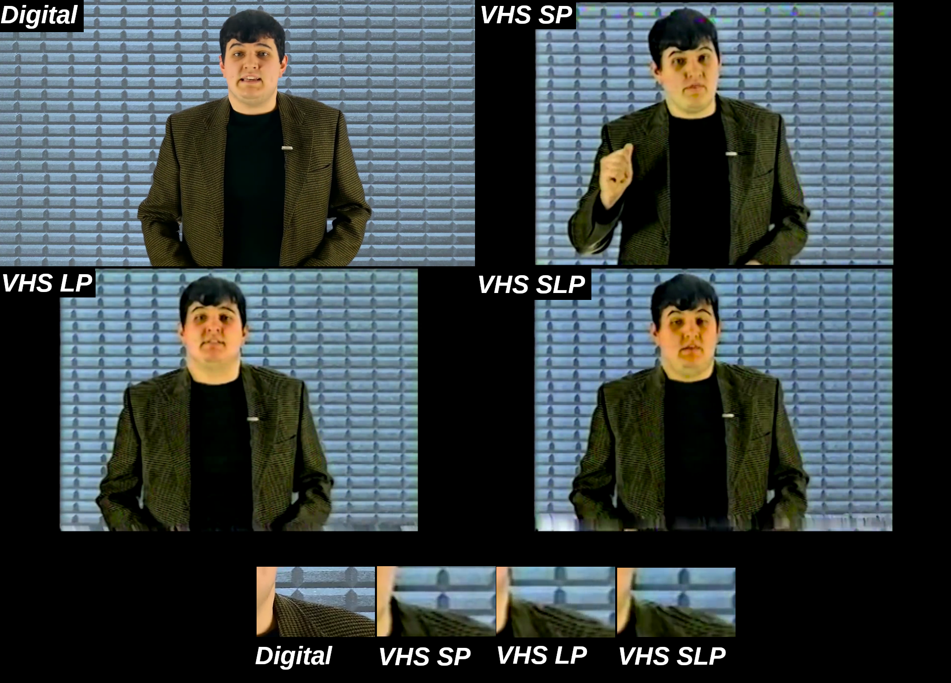
Video bandwidth comparison. Analogue broadcast - up to 6.5MHz, VHS SP - 3MHz,
VHS LP and SLP even less
Source: "The Impossible
Feat. inside your VCR" by Technology Connections
By running a convolution operation on each row on we can simulate a low-pass fiter that mimics the bandwidth limit of the cable. This operation results in blurring the image in the horizontal dimension
In order to run a convolution operation in numpy we first need a python function that will be ran on each row of the array
# This function is used to run convolution on a single row
def row_convolve(data, period):
    return np.convolve(data, np.ones((period,))/period, mode='valid')
Then we run if for each row in the array and normalize the data to be in the [0, 1] range
#Convolve and normalize
diff = np.apply_along_axis( lambda x: row_convolve(x, 5), axis=1, arr=diff )
diff *= 1/diff.max()
The result looks like this, like an LP, or even SLP VHS tape - they also used lower bandwidth (the result of slower tape speed to get more running time)

To model the signal reflection in the cable I decided to overlay the derivative of the data onto the original image, shifted slightly.
So first we need to define the shift function
#This function shifts the data in the array
def shift(data, dx, dy):
    n,m=data.shape
    bigdata=np.zeros((3*n,3*m),data.dtype)
    bigdata[n:2*n,m:2*m]=data
    x=n-dx
    y=m-dy
    return bigdata[x:x+n,y:y+m]
Then we need to make sure that we add two arrays of the same size, so we need a function that will expand a given array to a size (called shape in numpy) of another
def expand(source, targetshape):
    print("..expanding from " + str(source.shape) + " to " + str(targetshape.shape))
    return np.pad(source, ((targetshape.shape[0] - source.shape[0], 0),
    (targetshape.shape[1] - source.shape[1], 0) ), 'constant', constant_values=(0, 0))
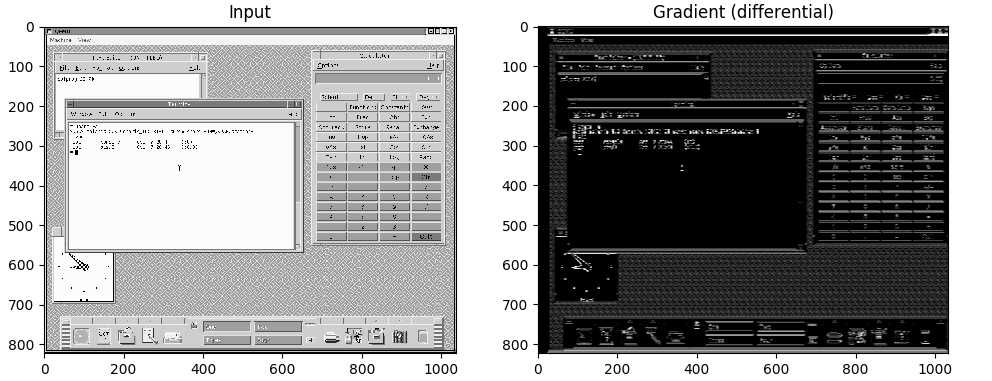
Then we can create an array that holds the differential of each row, or the gradient. Which we then take an absolute value of and shift a little, then convolve a bit to mimic a lowpass again
diff = shift(np.absolute(np.gradient(luma)[0]), 0, shiftpx)
#Convolve and normalize
diff = np.apply_along_axis( lambda x: row_convolve(x, 5), axis=1, arr=diff )
diff *= 1/diff.max()
diff = shift(diff, 0, shiftpx*2)
The diff array looks like this now
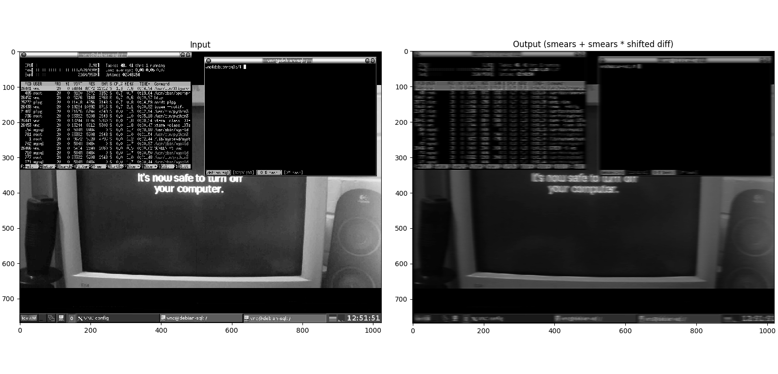
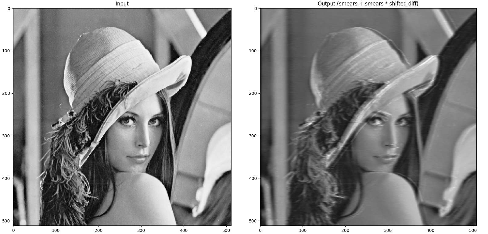
Then we can sum the low-passed data and the diff, in order to do this we need to match the size of the smear array. We normalize it as well
smear = expand(smear, diff)
smear *= 1/smear.max()

output = smear + smear*diff
We get this
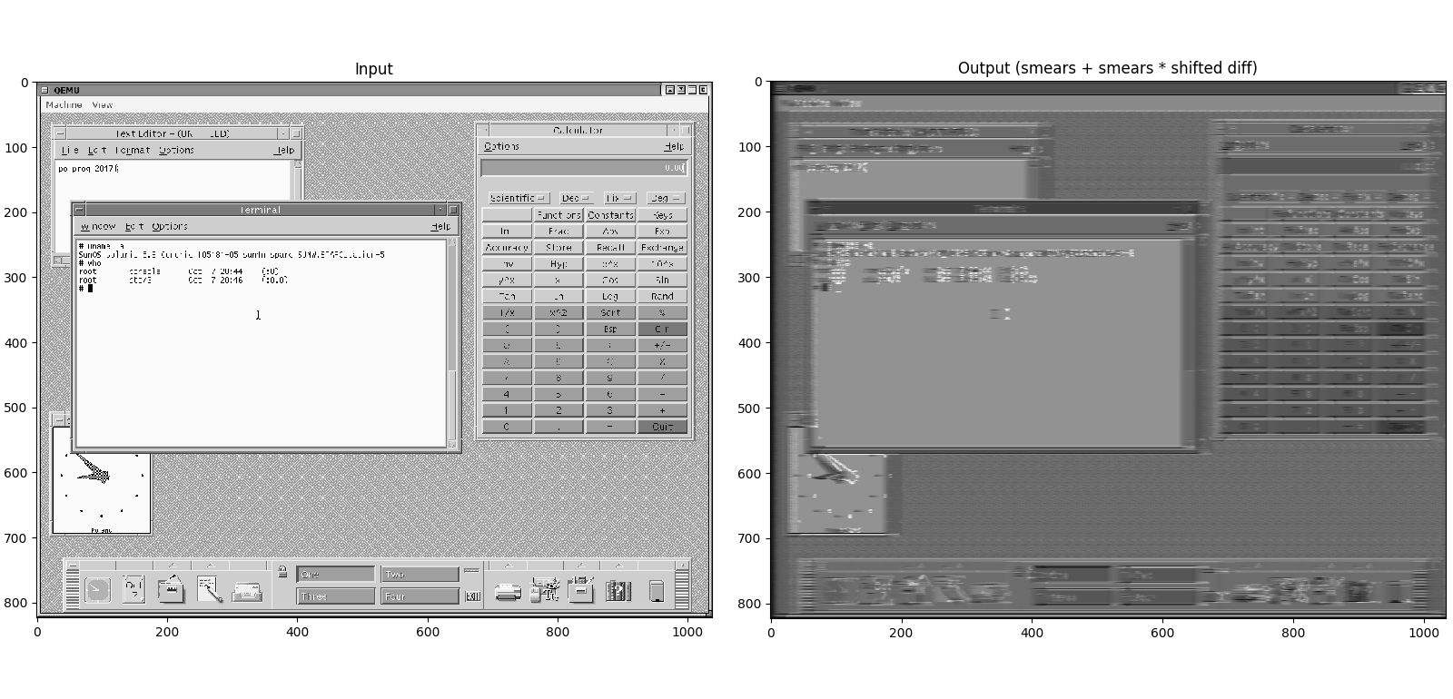
This image shows it step by step
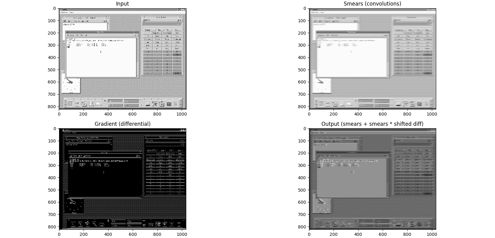
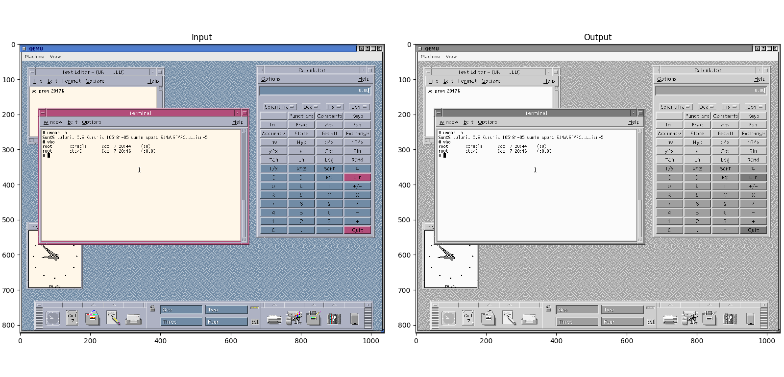
The script that generates it is the analogimage.py and twoimages.py
I think the script works best on screenshots

Here are some other outputs